General aspects
For individuals accustomed to prescribing boundary conditions directly at nodes—such as with Abaqus, Nastran input files, or Code-Aster command files—or even at geometric points, like in the MATLAB PDE Toolbox, transitioning to prescribe Dirichlet boundary conditions in FeniCSx can be challenging.
A basic understanding of finite element meshes and FEM function spaces is helpful, if not essential, for overcoming this challenge. It also proves invaluable when addressing other aspects of FeniCSx. A finite element mesh, also called grid, represents a discretization of a domain. It carries geometric and topological information, but it lacks details about the physics of the problem. Therefore, it is only one component of modeling a boundary value problem but, on the other hand, it can be used for different boundary value problems.
A finite element function space \(V_h\) consists of the mesh, a compatible interpolation basis, and information about the space’s dimension, dim(\(V_h\)). This dimension is dictated by the nature of the degrees of freedom (DOFs), which directly influence the definition of Dirichlet boundary conditions. For instance, in thermal problems, the DOFs are scalar values representing temperatures, whereas in continuum mechanics problems, the DOFs correspond to vectorial displacements.
Mesh information can be organized in various ways. A common approach, such as that used in Abaqus, involves defining the mesh through a node-coordinate list and an element-node list. In this context, the definition of \(V_h\) is implicit, as the chosen element type inherently includes details about the interpolation basis and the DOFs’ nature.
Finite element meshes are closely linked to graph theory since a mesh can be represented as a graph, enabling the application of graph-theoretical concepts for analysis and optimization. In three dimensions, a mesh hierarchy consists of objects of increasing dimension: vertices (dim = 0), edges (dim = 1), facets (dim = 2), and cells (dim = 3). Vertices and cells are often referred to as “nodes” and “volumes,” respectively. The relationships among these objects, independent of their geometry, define the topology of the mesh. In the context of Dirichlet boundary conditions, sets of boundary facets or edges are particularly useful. The geometry, however, is fully defined by the node-coordinate list (see, e.g., [1]).
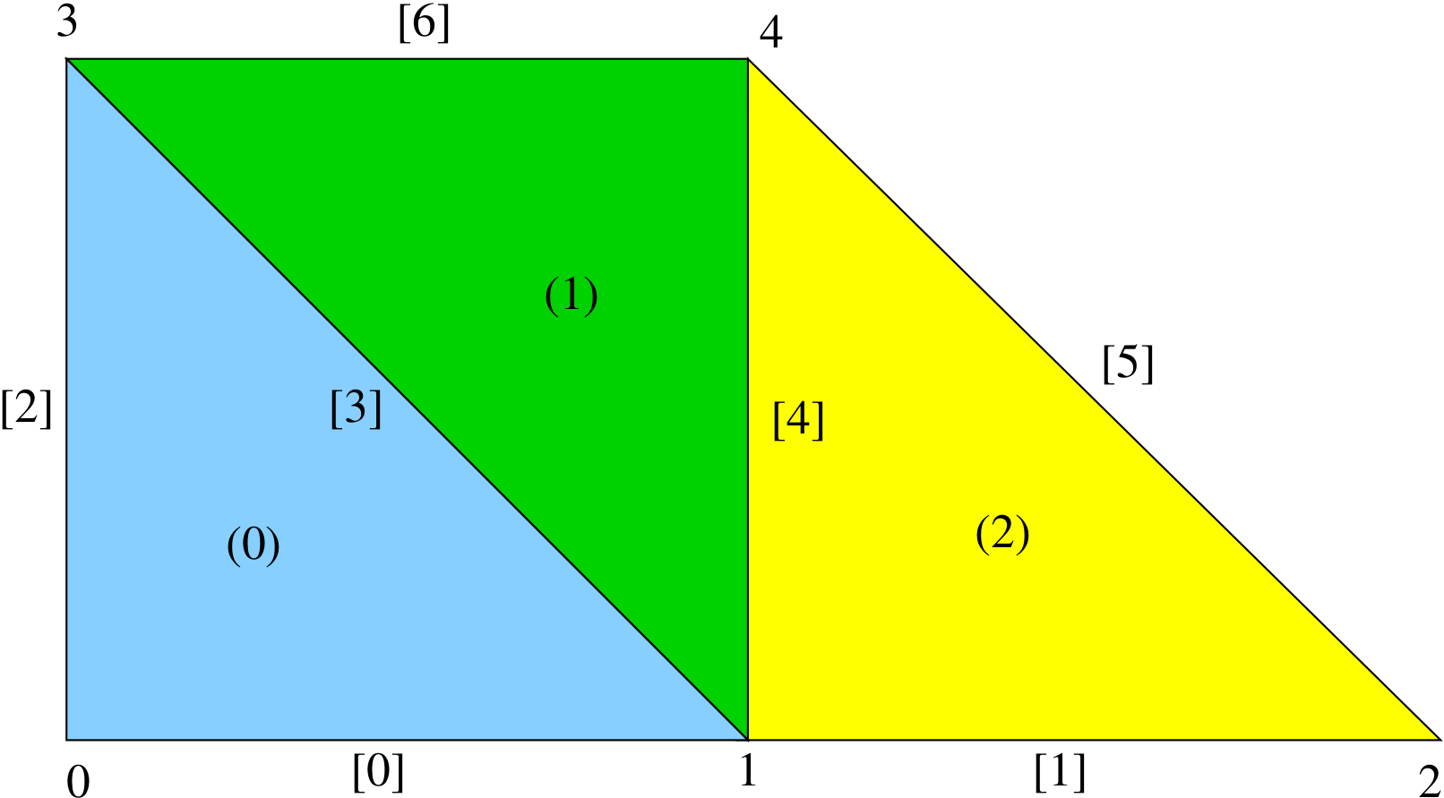
In two dimensions, cells have a dimensionality of two, and edges and facets coincide. Thus, the hierarchy simplifies to nodes (dim = 0), edges (dim = 1), and cells (dim= 2). All mesh information can be derived from a node-coordinate list, a cell-node list, and a specified order for defining the nodes of each cell.
To illustrate some of basic aspects, we consider the following two-dimensional mesh example.
Footnotes