Example Using SciPy and SLEPc for a Real Eigenvalue Problem

Problem

We analyze a beam-like structure clamped at one end, assuming a linear elastic material. This example demonstrates the use of the SciPy sparse solver as an alternative to, or in conjunction with, SLEPc.

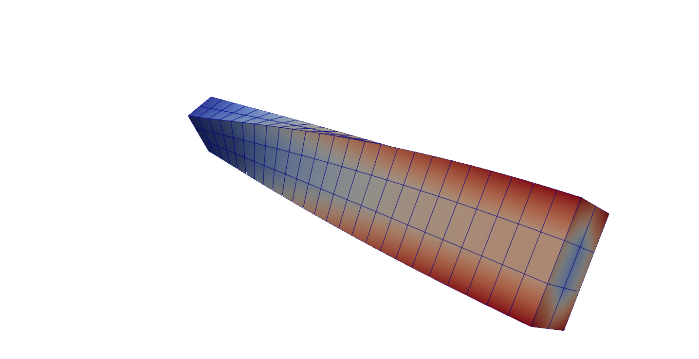
Fourth eigenmode of the beam-like structure clamped at one end (Paraview). The color corresponds to the magnitude of the displacement vector

Details of the Python Script

Note

You can download the complete python script TestModal.py

Import required libraries

import numpy as np
import ufl
import sys, slepc4py

slepc4py.init(sys.argv)

from dolfinx           import fem, mesh, io, default_scalar_type
from dolfinx.fem.petsc import assemble_matrix

from mpi4py     import MPI
from petsc4py   import PETSc
from slepc4py   import SLEPc

from scipy.sparse import csr_matrix
from scipy.sparse import linalg

This section imports the necessary libraries:

• dolfinx: For finite element computation.

• petsc4py and slepc4py: Interfaces for PETSc and SLEPc libraries for solving eigenvalue problems.

• scipy.sparse: For sparse matrix operations and solving eigenvalue problems with SciPy.

Define PETSc to SciPy Conversion Function

#--------------------------------------------------------------------
# FUNCTION FOR CONVERTING PETSc TO SciPy FORMAT
#--------------------------------------------------------------------
def PETSc2ScipySparse(PETScMatrix):
    """ converts a PETSc matrix to a SciPy sparse matrix """ 
  
    rows, cols        = PETScMatrix.getSize()                        # Get matrix dimensions
    ai, aj, av        = PETScMatrix.getValuesCSR()                   # Extract CSR data from PETSc matrix
    ScipySparseMatrix = csr_matrix((av, aj, ai), shape=(rows, cols)) # Create SciPy CSR matrix
    return(ScipySparseMatrix)

This function takes a PETSc sparse matrix and converts it to the SciPy csr_matrix format. This conversion is essential for compatibility when using SciPy’s eigenvalue solvers.

Define the Computational Domain and Mesh

#--------------------------------------------------------------------
# DOMAIN AND MESH
#--------------------------------------------------------------------    
L = np.array([5, 0.6, 0.4])
N = [25, 3, 2]
my_mesh = mesh.create_box(MPI.COMM_WORLD, [np.array([0,0,0]), L], N,
                          mesh.CellType.hexahedron)        

This block defines a 3D rectangular domain with dimensions [5, 0.6, 0.4] and a resolution of [25, 3, 2]. The mesh is created using Dolfinx and distributed across processors.

Define Material Properties and Constitutive Laws

#--------------------------------------------------------------------
# CONSTITUTIVE LAW (LINEAR ELASTICITY)
#--------------------------------------------------------------------
E, nu   = (2e11), (0.3)  
rho     = (7850) 
mu      = fem.Constant(my_mesh, E/2./(1+nu))
lamda   = fem.Constant(my_mesh, E*nu/(1+nu)/(1-2*nu))

def epsilon(u):
    return ufl.sym(ufl.grad(u))
def sigma(u):
    return lamda*ufl.nabla_div(u)*ufl.Identity(my_mesh.geometry.dim) + 2*mu*epsilon(u)

Defines material properties (Young’s modulus E, Poisson’s ratio nu, density rho) and constitutive relationships for linear elasticity:

• epsilon(u): Symmetric gradient (strain tensor).

• sigma(u): Stress tensor using the Lamé constants.

Define Function Space and Boundary Conditions

#--------------------------------------------------------------------
# FUNCTION SPACE, TRIAL AND TEST FUNCTION
#--------------------------------------------------------------------
V = fem.functionspace(my_mesh, ("CG", 1,(my_mesh.geometry.dim, )))
u = ufl.TrialFunction(V)
v = ufl.TestFunction(V)
#--------------------------------------------------------------------
# DIRICHLET BOUNDARY CONDITIONS
#--------------------------------------------------------------------
def clamped_boundary(x):
    return np.isclose(x[0], 0)

u_zero = np.array((0,) * my_mesh.geometry.dim, dtype=default_scalar_type)

bc = fem.dirichletbc(u_zero, fem.locate_dofs_geometrical(V, clamped_boundary), V)

• Creates a finite element function space for vector-valued functions.

• Implements Dirichlet boundary conditions (fixed at x=0).

Assemble Stiffness and Mass Matrices

#--------------------------------------------------------------------
# VARIATIONAL FORM, STIFFNESS AND MASS MATRIX
#--------------------------------------------------------------------
k_form = ufl.inner(sigma(u),epsilon(v))*ufl.dx
m_form = rho*ufl.inner(u,v)*ufl.dx
#
# Using the "diagonal" kwarg ensures that Dirichlet BC modes will not be among
# the lowest-frequency modes of the beam. 
K = fem.petsc.assemble_matrix(fem.form(k_form), bcs=[bc], diagonal=62831)
M = fem.petsc.assemble_matrix(fem.form(m_form), bcs=[bc], diagonal=1./62831)
K.assemble()
M.assemble()

Constructs stiffness (K) and mass (M) matrices from variational forms.

Solve Eigenvalue Problem with SciPy

#--------------------------------------------------------------------
# SciPy EIGENSOLVER 
#--------------------------------------------------------------------
KS = PETSc2ScipySparse(K)
MS = PETSc2ScipySparse(M)

num_eigenvs = 16
eigenvals, eigenvs = linalg.eigsh(KS, k=num_eigenvs, M=MS, which='SM')
SciPyFreqs         = np.sqrt(eigenvals.real)/2/np.pi

Converts the PETSc matrices to SciPy format and solves the generalized eigenvalue problem using the SciPy eigsh solver. The eigenvalues are converted to natural frequencies.

Solve Eigenvalue Problem with SLEPc

#--------------------------------------------------------------------
# SLEPc EIGENSOLVER 
#--------------------------------------------------------------------
#
# Create and configure eigenvalue solver
#
N_eig = 16
eigensolver = SLEPc.EPS().create(MPI.COMM_WORLD)

eigensolver.setDimensions(N_eig)
eigensolver.setProblemType(SLEPc.EPS.ProblemType.GHEP)

st = SLEPc.ST().create(MPI.COMM_WORLD)
st.setType(SLEPc.ST.Type.SINVERT)
st.setShift(0.1)
st.setFromOptions()
eigensolver.setST(st)
eigensolver.setOperators(K, M)
eigensolver.setFromOptions()
#
# Compute eigenvalue-eigenvector pairs
#
eigensolver.solve()

evs           = eigensolver.getConverged()
vr, vi        = K.getVecs()
#--------------------------------------------------------------------

• Configures and solves the eigenvalue problem using SLEPc.

• Applies spectral transformation (SINVERT) for improved convergence.

Output Results and Compare

# OUTPUT TO FILE AND COMPARISON
#--------------------------------------------------------------------
u_output      = fem.Function(V)
u_output.name = "Eigenvector"

print( "Number of converged eigenpairs %d" % evs )
if evs > 0:
    with io.XDMFFile(MPI.COMM_WORLD, "eigenvectors.xdmf", "w") as xdmf:
        xdmf.write_mesh(my_mesh)
        for i in range (min(N_eig, evs)):
            l = eigensolver.getEigenpair(i, vr, vi)
            freq = np.sqrt(l.real)/2/np.pi
            print(f"Mode {i}: {freq:.2f} Hz  {SciPyFreqs[i]:.2f} Hz")
            u_output.x.array[:] = vr
            xdmf.write_function(u_output, i)
                   
            

• Writes eigenvectors to an XDMF file for visualization.

• Compares the frequencies computed by SciPy and SLEPc. The results are printed for each mode.

Note

In case of an error message try first source dolfinx-real-mode in your Docker environment.